imported>Milton Beychok |
|
| Line 1: |
Line 1: |
| <u>'''This needs a lot of work yet'''</u><BR><BR>
| | {{AccountNotLive}} |
| | __NOTOC__ |
| | [[File:Crude oil-fired power plant.jpg|thumb|right|225px|Industrial air pollution source]] |
| | Atmospheric dispersion modeling is the mathematical simulation of how air pollutants disperse in the ambient atmosphere. It is performed with computer programs that solve the mathematical equations and algorithms which simulate the pollutant dispersion. The dispersion models are used to estimate or to predict the downwind concentration of air pollutants emitted from sources such as industrial plants, vehicular traffic or accidental chemical releases. |
|
| |
|
| '''Gasoline''' or '''petrol''' is derived from [[petroleum crude oil]]. Conventional gasoline is mostly a blended mixture of more than 200 different [[hydrocarbon]] [[liquid]]s ranging from those containing 4 [[carbon]] [[atom]]s to those containing 11 or 12 carbon atoms. It has an initial [[boiling point]] at [[atmospheric pressure]] of about 35 °[[Celsius|C]] (95 °[[Fahrenheit|F]]) and a final boiling point of about 200 °C (395 °F).<ref name=FAQ>[http://www.faqs.org/faqs/autos/gasoline-faq/part4/ Gasoline FAQ - Part2 of 4], Bruce Hamilton, Industrial Research Ltd. (IRL), a [[Crown Research Institute]] of [[New Zealand]].</ref><ref name=Gary>{{cite book|author=Gary, J.H. and Handwerk, G.E.|title=Petroleum Refining Technology and Economics|edition=4th Edition|publisher=Marcel Dekker, Inc.|year=2001|id=ISBN 0-8247-0482-7}}</ref><ref name=Assi>[http://hqweb.unep.org/pcfv/PDF/JordanWrkshp-Unleaded-Rafat.pdf The Relation Between Gasoline Quality, Octane Number and the Environment], Rafat Assi, National Project Manager of Jordan’s Second National Communications on Climate Change, Presented at Jordan National Workshop on Lead Phase-out, [[United Nations]] Environment Programme, July 2008, [[Amman]], [[Jordan]].</ref><ref>{{cite book|author=James Speight|title=Synthetic Fuels Handbook|edition=1st Edition|publisher=McGraw-Hill|pages=pages 92-93|year=2008|id=ISBN 0-07-149023-X}}</ref> Gasoline is used primarily as fuel for the [[internal combustion engine]]s in automotive vehicles as well in some small airplanes.
| | Such models are important to governmental agencies tasked with protecting and managing the ambient air quality. The models are typically employed to determine whether existing or proposed new industrial facilities are or will be in compliance with the National Ambient Air Quality Standards (NAAQS) in the United States or similar regulations in other nations. The models also serve to assist in the design of effective control strategies to reduce emissions of harmful air pollutants. During the late 1960's, the Air Pollution Control Office of the U.S. Environmental Protection Agency (U.S. EPA) initiated research projects to develop models for use by urban and transportation planners.<ref>J.C. Fensterstock et al, "Reduction of air pollution potential through environmental planning", ''JAPCA'', Vol. 21, No. 7, 1971.</ref> |
| | |
| In [[Canada]] and the [[United States]], the word "gasoline" is commonly used and it is often shortened to simply "gas" although it is a liquid rather than a [[gas]]. In fact, gasoline-dispensing facilities are referred to as "gas stations".
| |
|
| |
|
| Most current or former [[Commonwealth of Nations|Commonwealth countries]] use the term "petrol" and dispensing facilities are referred to as "petrol stations". The term "petrogasoline" is also used sometimes. In some European countries and elsewhere, the term "benzin" (or a variant of that word) is used to denote gasoline.
| | Air dispersion models are also used by emergency management personnel to develop emergency plans for accidental chemical releases. The results of dispersion modeling, using worst case accidental releases and meteorological conditions, can provide estimated locations of impacted areas and be used to determine appropriate protective actions. At industrial facilities in the United States, this type of consequence assessment or emergency planning is required under the Clean Air Act (CAA) codified in Part 68 of Title 40 of the Code of Federal Regulations. |
|
| |
|
| In aviation, "mogas" (short for "motor gasoline") is used to distinguish automotive vehicle fuel from aviation fuel known as "avgas".
| | The dispersion models vary depending on the mathematics used to develop the model, but all require the input of data that may include: |
|
| |
|
| == Gasoline production from crude oil ==
| | * Meteorological conditions such as wind speed and direction, the amount of atmospheric turbulence (as characterized by what is called the "stability class"), the ambient air temperature, the height to the bottom of any inversion aloft that may be present, cloud cover and solar radiation. |
| | * The emission parameters such the type of source (i.e., point, line or area), the mass flow rate, the source location and height, the source exit velocity, and the source exit temperature. |
| | * Terrain elevations at the source location and at receptor locations, such as nearby homes, schools, businesses and hospitals. |
| | * The location, height and width of any obstructions (such as buildings or other structures) in the path of the emitted gaseous plume as well as the terrain surface roughness (which may be characterized by the more generic parameters "rural" or "city" terrain). |
|
| |
|
| {{Image|Refinery Products Barrel.png|right|250px|Average U.S. refinery product yields.}}
| | Many of the modern, advanced dispersion modeling programs include a pre-processor module for the input of meteorological and other data, and many also include a post-processor module for graphing the output data and/or plotting the area impacted by the air pollutants on maps. The plots of areas impacted usually include isopleths showing areas of pollutant concentrations that define areas of the highest health risk. The isopleths plots are useful in determining protective actions for the public and first responders. |
|
| |
|
| Gasoline and other end-products are produced from petroleum crude oil in [[Petroleum refining processes|petroleum refineries]]. It is very difficult to quantify the amount of gasoline produced by refining a given amount of crude oil for a number of reasons:
| | The atmospheric dispersion models are also known as atmospheric diffusion models, air dispersion models, air quality models, and air pollution dispersion models. |
|
| |
|
| * There are quite literally hundreds of different crude oil sources worldwide and each crude oil has its own unique mixture of thousands of hydrocarbons and other materials.
| | ==Atmospheric layers== |
|
| |
|
| * There are also hundreds of crude oil refineries worldwide and each of them is designed to process a specific crude oil or a specific set of crude oils. Furthermore, each refinery has its own unique configuration of [[petroleum refining processes]] that produces its own unique set of gasoline blend components.
| | Discussion of the layers in the Earth's atmosphere is needed to understand where airborne pollutants disperse in the atmosphere. The layer closest to the Earth's surface is known as the ''troposphere''. It extends from sea-level up to a height of about 18 km and contains about 80 percent of the mass of the overall atmosphere. The ''stratosphere'' is the next layer and extends from 18 km up to about 50 km. The third layer is the ''mesosphere'' which extends from 50 km up to about 80 km. There are other layers above 80 km, but they are insignificant with respect to atmospheric dispersion modeling. |
|
| |
|
| * There are a great many different gasoline specifications that have been mandated by various local, state or national governmental agencies.
| | The lowest part of the troposphere is called the ''atmospheric boundary layer (ABL)'' or the ''planetary boundary layer (PBL)'' and extends from the Earth's surface up to about 1.5 to 2.0 km in height. The air temperature of the atmospheric boundary layer decreases with increasing altitude until it reaches what is called the ''inversion layer'' (where the temperature increases with increasing altitude) that caps the atmospheric boundary layer. The upper part of the troposphere (i.e., above the inversion layer) is called the ''free troposphere'' and it extends up to the 18 km height of the troposphere. |
|
| |
|
| * In many geographical areas, the amount of gasoline produced during the summer season (i.e., the season of the greatest demand for automotive gasoline) varies significantly from the amount produced during the winter season.
| | The ABL is the most important layer with respect to the emission, transport and dispersion of airborne pollutants. The part of the ABL between the Earth's surface and the bottom of the inversion layer is known as the ''mixing layer''. Almost all of the airborne pollutants emitted into the ambient atmosphere are transported and dispersed within the mixing layer. Some of the emissions penetrate the inversion layer and enter the free troposphere above the ABL. |
|
| |
|
| However, from the data presented in the adjacent image as an average of all the refineries operating in the United States in 2007,<ref name=EIA-Products>[http://www.eia.doe.gov/bookshelf/brochures/gasoline/index.html Where Does My Gasoline Come from?], [[U.S. Department of Energy]], [[Energy Information Administration]], April 2008.</ref> refining a barrel of crude oil (i.e., 42 [[U.S. customary units|gallons]] or 159 [[litre]]s) yielded 19.2 gallons (72.7 litres) of end-product gasoline. That is a volumetric yield of 45.7 percent. The average refinery yield of gasoline in other countries may be different.
| | In summary, the layers of the Earth's atmosphere from the surface of the ground upwards are: the ABL made up of the mixing layer capped by the inversion layer; the free troposphere; the stratosphere; the mesosphere and others. Many atmospheric dispersion models are referred to as ''boundary layer models'' because they mainly model air pollutant dispersion within the ABL. To avoid confusion, models referred to as ''mesoscale models'' have dispersion modeling capabilities that can extend horizontally as much as a few hundred kilometres. It does not mean that they model dispersion in the mesosphere. |
|
| |
|
| From a marketing viewpoint, the most important characteristic of a gasoline is its [[octane number]] (discussed later in this article). [[Paraffin|Paraffinic hydrocarbons]] ([[alkane]]s) wherein all of the carbon atoms are in a straight chain have the lowest octane numbers. Hydrocarbons with more complicated configurations such as [[aromatic]]s, [[olefin]]s and highly branched [[paraffin]]s have much higher octane numbers. To that end, many of the refining processes used in petroleum refineries are designed to produce hydrocarbons with those more complicated configurations.
| | ==Gaussian air pollutant dispersion equation== |
|
| |
|
| Some of the most important refinery process streams that are blended together to obtain the end-product gasolines<ref>See the schematic flow diagram in the [[Petroleum refining processes]] article.</ref> are:
| | The technical literature on air pollution dispersion is quite extensive and dates back to the 1930s and earlier. One of the early air pollutant plume dispersion equations was derived by Bosanquet and Pearson.<ref>C.H. Bosanquet and J.L. Pearson, "The spread of smoke and gases from chimneys", ''Trans. Faraday Soc.'', 32:1249, 1936.</ref> Their equation did not assume Gaussian distribution nor did it include the effect of ground reflection of the pollutant plume. |
|
| |
|
| *''Reformate'' (produced in a [[Catalytic reforming|catalytic reformer]]): has a high content of aromatic hydrocarbons and a very low content of olefinic hydrocarbons ([[alkene]]s).
| | Sir Graham Sutton derived an air pollutant plume dispersion equation in 1947<ref>O.G. Sutton, "The problem of diffusion in the lower atmosphere", ''QJRMS'', 73:257, 1947.</ref><ref>O.G. Sutton, "The theoretical distribution of airborne pollution from factory chimneys", ''QJRMS'', 73:426, 1947.</ref> which did include the assumption of Gaussian distribution for the vertical and crosswind dispersion of the plume and also included the effect of ground reflection of the plume. |
| *''Catalytically cracked gasoline'' (produced in a [[Fluid catalytic cracking|fluid catalytic cracker]]): has a high content of olefinic hydrocarbons and a moderate amount of aromatic hydrocarbons.
| |
| *''Hydrocrackate'' (produced in a [[Hydrocracking|hydrocracker]]): has a moderate content of aromatic hydrocarbons.
| |
| *''Alkylate'' (produced in an [[Alkylation process|alkylation unit]]): has a high content of highly branched paraffinic hydrocarbons such as [[isooctane]].
| |
| *''Isomerate'' (produced in a [[Catalytic isomerization|catalytic isomerization unit]]): has a high content of the branched [[isomers]] of [[pentane]] and [[hexane]].
| |
|
| |
|
| == Gasoline formulations and air quality regulations == | | Under the stimulus provided by the advent of stringent environmental control regulations, there was an immense growth in the use of air pollutant plume dispersion calculations between the late 1960s and today. A great many computer programs for calculating the dispersion of air pollutant emissions were developed during that period of time and they were commonly called "air dispersion models". The basis for most of those models was the '''Complete Equation For Gaussian Dispersion Modeling Of Continuous, Buoyant Air Pollution Plumes''' shown below:<ref name=Beychok>{{cite book|author=M.R. Beychok|title=Fundamentals Of Stack Gas Dispersion|edition=4th Edition| publisher=author-published|year=2005|isbn=0-9644588-0-2}}.</ref><ref>{{cite book|author=D. B. Turner| title=Workbook of atmospheric dispersion estimates: an introduction to dispersion modeling| edition=2nd Edition |publisher=CRC Press|year=1994|isbn=1-56670-023-X}}.</ref> |
|
| |
|
| === In the United States ===
| |
|
| |
|
| There is no "standard" composition or set of specifications for gasoline. In the United States, because of the complex national and individual state and local programs to improve air quality, as well as local refining and marketing decisions, petroleum refiners must supply fuels that meet many different standards. State and local air quality regulations involving gasoline overlap with national regulations and that leads to adjacent or nearby areas having significantly different gasoline specifications. According to a detailed study in 2006, <ref name=CRS>[http://www.scribd.com/doc/1537932/US-Air-Force-rl31361 CRS Report For Congress] ''"Boutique Fuels" and Reformulated Gasoline: Harmonization of Fuel Standards'' (May 10, 2006) , Brent D. Yacobucci, Congressional Research Service, [[Library of Congress]]</ref> there were at least 18 different gasoline formulations required across the United States in 2002. Since many petroleum refiners in the United States produce three grades of fuel and the specifications for fuel marketed in the summer season vary significantly from the specifications in the winter season, that number may have been greatly understated. In any event, the number of fuel formulations has probably increased quite a bit since 2002. In the United States, the various fuel formulations are often referred to as "boutique fuels".<ref name=CRS/><ref>[http://www.epa.gov/oms/boutique.htm Boutique Fuels: State and Local Clean Fuels Programs] From the website of the [[U.S. Environmental Protection Agency]]</ref><ref>[http://www.epa.gov/oms/boutique/420r06901.pdf EPAct Section 1541 Boutique Fuels Report to Congress] Report No. EPA420-R-06-901, December 2006, co-authored by the U.S. EPA and the [[U.S. Department of Energy]].</ref> In general, most of the gasoline specifications meet the requirements of the so-called '''''Reformulated Gasoline (RFG)''''' mandated by federal law and implemented by the [[U.S. Environmental Protection Agency]] (U.S. EPA).
| | <math>C = \frac{\;Q}{u}\cdot\frac{\;f}{\sigma_y\sqrt{2\pi}}\;\cdot\frac{\;g_1 + g_2 + g_3}{\sigma_z\sqrt{2\pi}}</math> |
|
| |
|
| Some of the major properties and gasoline components focused upon by the various national and state or local regulatory programs are:
| | {| border="0" cellpadding="2" |
| | |- |
| | |align=right|where: |
| | | |
| | |- |
| | !align=right|<math>f</math> |
| | |align=left|= crosswind dispersion parameter |
| | |- |
| | !align=right| |
| | |align=left|= <math>\exp\;[-\,y^2/\,(2\;\sigma_y^2\;)\;]</math> |
| | |- |
| | !align=right|<math>g</math> |
| | |align=left|= vertical dispersion parameter = <math>\,g_1 + g_2 + g_3</math> |
| | |- |
| | !align=right|<math>g_1</math> |
| | |align=left|= vertical dispersion with no reflections |
| | |- |
| | !align=right| |
| | |align=left|= <math>\; \exp\;[-\,(z - H)^2/\,(2\;\sigma_z^2\;)\;]</math> |
| | |- |
| | !align=right|<math>g_2</math> |
| | |align=left|= vertical dispersion for reflection from the ground |
| | |- |
| | !align=right| |
| | |align=left|= <math>\;\exp\;[-\,(z + H)^2/\,(2\;\sigma_z^2\;)\;]</math> |
| | |- |
| | !align=right|<math>g_3</math> |
| | |align=left|= vertical dispersion for reflection from an inversion aloft |
| | |- |
| | !align=right| |
| | |align=left|= <math>\sum_{m=1}^\infty\;\big\{\exp\;[-\,(z - H - 2mL)^2/\,(2\;\sigma_z^2\;)\;]</math> |
| | |- |
| | !align=right| |
| | |align=left| <math>+\, \exp\;[-\,(z + H + 2mL)^2/\,(2\;\sigma_z^2\;)\;]</math> |
| | |- |
| | !align=right| |
| | |align=left| <math>+\, \exp\;[-\,(z + H - 2mL)^2/\,(2\;\sigma_z^2\;)\;]</math> |
| | |- |
| | !align=right| |
| | |align=left| <math>+\, \exp\;[-\,(z - H + 2mL)^2/\,(2\;\sigma_z^2\;)\;]\big\}</math> |
| | |- |
| | !align=right|<math>C</math> |
| | |align=left|= concentration of emissions, in g/m³, at any receptor located: |
| | |- |
| | !align=right| |
| | |align=left| x meters downwind from the emission source point |
| | |- |
| | !align=right| |
| | |align=left| y meters crosswind from the emission plume centerline |
| | |- |
| | !align=right| |
| | |align=left| z meters above ground level |
| | |- |
| | !align=right|<math>Q</math> |
| | |align=left|= source pollutant emission rate, in g/s |
| | |- |
| | !align=right|<math>u</math> |
| | |align=left|= horizontal wind velocity along the plume centerline, m/s |
| | |- |
| | !align=right|<math>H</math> |
| | |align=left|= height of emission plume centerline above ground level, in m |
| | |- |
| | !align=right|<math>\sigma_z</math> |
| | |align=left|= vertical standard deviation of the emission distribution, in m |
| | |- |
| | !align=right|<math>\sigma_y</math> |
| | |align=left|= horizontal standard deviation of the emission distribution, in m |
| | |- |
| | !align=right|<math>L</math> |
| | |align=left|= height from ground level to bottom of the inversion aloft, in m |
| | |- |
| | !align=right|<math>\exp</math> |
| | |align=left|= the exponential function |
| | |} |
|
| |
|
| *''[[Vapor pressure]]'': The vapor pressure of a gasoline is a measure of its propensity to evaporate. Evaporative [[emission]]s of the hydrocarbons in the gasoline lead to the formation of [[ozone]] in the atmosphere which reacts with vehicular and industrial emissions of gaseous [[nitrogen oxides]] (NOx) to form what is called ''[[photochemical smog]]''. ''Smog'' is a combination of the words ''smoke '' and ''fog'' and traditionally referred to the mixture of smoke and [[sulfur dioxide]] that resulted from the burning of coal for heating buildings in places such as [[London]], [[England]]. Modern photochemical smog does not come from coal burning but from vehicular and industrial emissions of hydrocarbons and nitrogen oxides. It appears as a brownish haze over large urban areas and is irritating to the eyes and lungs.
| | The above equation not only includes upward reflection from the ground, it also includes downward reflection from the bottom of any inversion lid present in the atmosphere. |
|
| |
|
| *''Nitrogen oxides'': Various nitrogen oxides (NOx) are formed during the combustion of gasoline in vehicles and the combustion of other fuels in industrial facilities. NOx is one of the ingredients involved in the atmospheric chemistry that produces photochemical smog and, as such, is a prominent air pollutant. In fact, it is one of the six so-called "criteria air pollutants" that are regulated by [[National Ambient Air Quality Standards]] (NAAQS) of the United States. The NOx emitted by vehicular engines using gasoline are largely controlled by the use of on-board devices, called [[catalytic converter]]s, installed on most modern automobiles and other vehicles. They convert the NOx emissions into gaseous [[nitrogen]] and [[oxygen]]. They also convert any gaseous [[carbon monoxide]] emissions into [[carbon dioxide]] as well as converting any unburnt gasoline hydrocarbons into carbon dioxide and water [[vapor]].
| | The sum of the four exponential terms in <math>g_3</math> converges to a final value quite rapidly. For most cases, the summation of the series with '''''m''''' = 1, '''''m''''' = 2 and '''''m''''' = 3 will provide an adequate solution. |
|
| |
|
| *''Toxic metals'':
| | <math>\sigma_z</math> and <math>\sigma_y</math> are functions of the atmospheric stability class (i.e., a measure of the turbulence in the ambient atmosphere) and of the downwind distance to the receptor. The two most important variables affecting the degree of pollutant emission dispersion obtained are the height of the emission source point and the degree of atmospheric turbulence. The more turbulence, the better the degree of dispersion. |
| **''[[Tetra-ethyl lead]] (TEL)'' — In the 1920's, petroleum refining technology was rather primitive and produced gasolines with an octane number of about 40 – 60. But automotive engines were rapidly being improved and required better gasolines, which led to a search for octane enhancers. That search culminated in 1924 in the development and widespread usage of tetra-ethyl lead (TEL), a colorless, viscous liquid with the chemical formula of (CH<sub>3</sub>CH<sub>2</sub>)<sub>4</sub>Pb. TEL became commercially available as what was called ''TEL fluid'', which contained 61.5 weight % TEL. The addition of as little as 0.8 ml of that TEL fluid per [[litre]] (equivalent to 0.5 gram of lead per litre) of gasoline resulted in significant octane number increases. For about the next 50 years, TEL was used as the most cost effective way to raise the octane number of gasolines. During that period, petroleum refining technology grew until high-octane gasolines could, in fact, be produced without using TEL. Also, in about the 1940's, it was discovered that the lead being emitted in the exhaust gases from vehicular internal combustion engines was a toxic air pollutant that seriously affected human health. Because of its toxicity and the fact that catalytic converters being installed in vehicles could not tolerate the presence of lead, the U.S. EPA launched an initiative in 1972 to phase out the use of TEL in the United States and it was completely banned for use in on-road vehicles as of January 1996.<ref>[http://www.uneptie.org/energy/transport/documents/pdf/phasingLead.pdf Phasing Lead Out of Gasoline] a report issued by the [[United Nations Environmental Programme]] (UNEP)</ref> <ref>[http://www.epa.gov/EPA-AIR/1996/February/Day-02/pr-1326.html Prohibition on Gasoline Containing Lead or Lead Additives for Highway Use] From the website of the U.S. Environmental Protection Agency</ref> Using TEL in race cars, airplanes, marine engines and farm equipment is still permitted. TEL usage has also been phased out by most nations worldwide. As of 2008, the only nations still allowing extensive use of TEL are the [[Democratic People's Republic of Korea]], [[Myanamar]], and [[Yeman]].<ref>[http://www.unep.org/pcfv/PDF/LeadMatrix-Asia-PacificAug08.pdf Asia-Pacific Lead Matrix] a report issued by the United Nations Environmental Programme (UNEP)</ref><ref>[http://www.unep.org/pcfv/PDF/MatrixMENAWAJan07.pdf West Asia, Middle East and North Africa Lead Matrix] a report issued by the United Nations Environmental Programme (UNEP)</ref>
| |
| **''[[Methylcyclopentadienyl manganese tricarbonyl]] (MMT)'' — In [[Canada]], MMT has been used as an octane enhancer in gasoline since 1976. It is also permitted for use as a gasoline octane enhancer in [[Argentina]], [[Australia]], [[Bulgaria]], [[France]], [[Russia]], United States and conditionally in [[New Zealand]]. MMT is a yellow liquid with chemical formula of (CH<sub>3</sub>C<sub>5</sub>H<sub>4</sub>)Mn(CO)<sub>3</sub>. According to the U.S. EPA, ingested [[manganese]] is a required element of the diet at very low levels but it is also a [[neurotoxin]] and can cause irreversible neurological disease at high levels of inhalation.<ref name=EPAMMT>[http://www.epa.gov/otaq/regs/fuels/additive/mmt_cmts.htm Comments on the Gasoline Additive MMT] Retrieved from the U.S. EPA website on April 10, 2009</ref> The U.S. EPA has a concern that the use of MMT in gasoline could increase inhalation manganese exposures. After completing a 1994 risk evaluation on the use of MMT in gasoline, the U.S. EPA was unable to determine if there is a risk to the public health from exposure to emissions of MMT gasoline. As of now (2009), gasoline in the United States is allowed to contain MMT at a level equivalent to 0.00826 g/L (1/32 g/gallon) of manganese.<ref name=EPAMMT/> However, there are still many concerns about the possible adverse health effects from the usage of MMT and less than one percent of the gasoline marketed in the United States contains MMT.<ref name=ICCT>[http://www.theicct.org/documents/MMT_ICCT_2009.pdf Methylcyclopentadienyl Manganese Tricarbonyl (MMT): A Science and Policy Review] Published by the International Council on Clean Transportation, January 2009</ref>
| |
|
| |
|
| *''Other toxic compounds'': Gasoline contains some [[benzene]] (C<sub>6</sub>H<sub>6</sub>) which is an aromatic compound that is a known human [[carcinogen]]. For that reason, the amount of benzene in gasoline is limited by environmental regulations. In general, the combustion of aromatics can lead to the formation of other compounds that have deleterious effects on human health, such as [[aldehyde]]s, [[butadiene]], and [[polycylclic aromatic hydrocarbon]]s (PAHs). Therefore, the total amount of aromatics in gasoline is also limited by environmental regulations.
| | Whereas older models rely on stability classes for the determination of <math>\sigma_y</math> and <math>\sigma_z</math>, more recent models increasingly rely on Monin-Obukhov similarity theory to derive these parameters. |
|
| |
|
| *''Olefins'': Photochemical smog is formed by various atmospheric chemistry reactions between nitrogen oxides and waht are called ''reactive hydrocarbons'' in the presence of sunlight. In the context of photochemical smog formation, some hydrocarbons are more reactive than others. For example, olefins are very reactive and methane is not reactive to any extent. For that reason, the olefin content of gasolines is limited by environmental regulations.
| | ==Briggs plume rise equations== |
|
| |
|
| *''[[Sulfur]]'': Any sulfur compounds in gasoline will result in combustion exhaust emissions of sulfur dioxide to the atmosphere. Such emissions contribute to the formation of so-called ''[[acid rain]]'' and they also interfere with the on-board catalytic converters and reduce their efficiency. Therefore, the sulfur content of gasolines is limited by environmental regulations.
| | The Gaussian air pollutant dispersion equation (discussed above) requires the input of ''H'' which is the pollutant plume's centerline height above ground level. ''H'' is the sum of ''H''<sub>s</sub> (the actual physical height of the pollutant plume's emission source point) plus Δ''H'' (the plume rise due the plume's buoyancy). |
|
| |
|
| *''Oxygen'': Oxygen-containing compounds called [[oxygenate]]s such as [[ethanol]] (with a chemical formula of C<sub>2</sub>H<sub>5</sub>OH) or [[methyl tertiary-butyl ether]] (MTBE) (with a chemical formula of C<sub>5</sub>H<sub>12</sub>O) are added to gasolines for two reasons. The first reason is that the oxygen reduces the emissions of unburnt hydrocarbons as well as the emissions of carbon monoxide. The second reason is that they significantly enhance the octane number of gasolines which makes up for the octane number loss resulting from the limiting of the high-octane number aromatics and olefins as well as the banning of TEL usage.<ref name=Gary/> MTBE was widely used during the 1990s as an oxygenate in the United States until it was found to be polluting underground water supplies. In the United States, it has now been largely replaced as an oxygenate by ethanol.
| | [[File:Gaussian Plume.png|thumb|right|333px|Visualization of a buoyant Gaussian air pollutant dispersion plume]] |
|
| |
|
| As mentioned earlier above, there are a great many different sets of specifications or standards for gasolines marketed in the United States. The specifications tabulated below are those that have been mandated by law in in the state of [[California]]. They are known as the '''''California Reformulated Gasoline (CaRFG)''''' Phase 3 Standards and are perhaps the most environmentally restrictive specifications in the United States:
| | To determine Δ''H'', many if not most of the air dispersion models developed between the late 1960s and the early 2000s used what are known as "the Briggs equations." G.A. Briggs first published his plume rise observations and comparisons in 1965.<ref>G.A. Briggs, "A plume rise model compared with observations", ''JAPCA'', 15:433–438, 1965.</ref> In 1968, at a symposium sponsored by CONCAWE (a Dutch organization), he compared many of the plume rise models then available in the literature.<ref>G.A. Briggs, "CONCAWE meeting: discussion of the comparative consequences of different plume rise formulas", ''Atmos. Envir.'', 2:228–232, 1968.</ref> In that same year, Briggs also wrote the section of the publication edited by Slade<ref>D.H. Slade (editor), "Meteorology and atomic energy 1968", Air Resources Laboratory, U.S. Dept. of Commerce, 1968.</ref> dealing with the comparative analyses of plume rise models. That was followed in 1969 by his classical critical review of the entire plume rise literature,<ref>G.A. Briggs, "Plume Rise", ''USAEC Critical Review Series'', 1969.</ref> in which he proposed a set of plume rise equations which have become widely known as "the Briggs equations". Subsequently, Briggs modified his 1969 plume rise equations in 1971 and in 1972.<ref>G.A. Briggs, "Some recent analyses of plume rise observation", ''Proc. Second Internat'l. Clean Air Congress'', Academic Press, New York, 1971.</ref><ref>G.A. Briggs, "Discussion: chimney plumes in neutral and stable surroundings", ''Atmos. Envir.'', 6:507–510, 1972.</ref> |
|
| |
|
| {| class = "wikitable" align="center"
| | Briggs divided air pollution plumes into these four general categories: |
| |+ California Reformulated Gasoline (CaRFG) Phase 3 Standards<ref>[http://www.arb.ca.gov/fuels/gasoline/carfg/082908.pdf Final Regulation Order] 2007 Amendments to California Phase 3 Reformulated Gasoline Regulation, California Code of Regulations, Title 13, Section 2260</ref><br>Effective as of August 29, 2008<ref>[http://www.arb.ca.gov/fuels/gasoline/carfg3/carfg3.htm California Phase 3 Reformulated Gasoline (CaRFG)]</ref>
| | * Cold jet plumes in calm ambient air conditions |
| ! Property!!Measurement<br>unit!!Flat Limit<sup> (a)</sup>!!Average Limit<sup> (a)</sup>
| | * Cold jet plumes in windy ambient air conditions |
| |- align="center"
| | * Hot, buoyant plumes in calm ambient air conditions |
| |[[Reid vapor pressure]]<sup> (b)</sup>||[[U.S. customary units|psi]]<sup> (c)</sup>||7.00 or 6.90<sup> (d)</sup> ||not applicable
| | * Hot, buoyant plumes in windy ambient air conditions |
| |- align="center"
| |
| |Sulfur [[concentration]]||[[Parts per notation|ppmw]]||20||15
| |
| |- align="center"
| |
| |Benzene concentration||[[Parts per notation|ppmv]]||0.8||0.7
| |
| |- align="center"
| |
| |Aromatics concentration||ppmv||25.0 ||22.0
| |
| |- align="center"
| |
| |Olefins concentration||ppmv||6.0 ||4.0
| |
| |- align="center"
| |
| |[[Temperature]] at 50 [[Concentration|volume %]] distilled (T50)||°F<sup> (e)</sup>||213||203
| |
| |- align="center"
| |
| |Temperature at 90 volume % distilled (T90)||°F||305||295
| |
| |- align="center"
| |
| |Oxygen concentration||[[Concentration|weight]] %<sup> (f)</sup>||1.8 – 2.2 ||not applicable
| |
| |- align="center"
| |
| |Oxygenates other than ethanol||--||prohibited||not applicable
| |
| |-
| |
| |colspan=4|(a)"Flat" limits apply to every batch of finished gasoline. "Average" limits allow specific batches to<br>exceed the "flat" limits as long as the gasoline produced over a 180-day period meets the "average"<br>limits and never exceeds the specified "cap" limits.<br>
| |
| (b) Reid vapor pressure (RVP) is measured as per [[ASTM]] method D-323 and differs slightly from the true<br>absolute [[vapor pressure]].<br>
| |
| (c) 1 psi = 6.89 k[[Pascal (unit)|Pa]]<br>
| |
| (d) The Reid vapor pressure flat limit of 6.90 psi applies when a California gasoline producer or importer<br> uses the CaRFG Phase 3 Predictive Model to certify a gasoline blend not containing ethanol. Otherwise,<br> the 7.0 psi limit applies.<br>
| |
| (e) °C = (°F − 32)(5/9) <br>
| |
| (f) Volume % ethanol in gasoline = [(0.3529/weight % oxygen) − 0.0006]<sup> −1</sup>. Thus, 1.8 – 2.2 weight %<br>oxygen in a gasoline equals 5.1 – 6.3 volume % ethanol in the gasoline.<ref>[http://www.arb.ca.gov/regact/mtbepost/appe.PDF Miscellaneous Cleanup Amendments to the California Reformulated Gasoline Regulations]</ref>
| |
| |}
| |
|
| |
|
| ====Blendstock for Oxygenate Blending (BOB)====
| | Briggs considered the trajectory of cold jet plumes to be dominated by their initial velocity momentum, and the trajectory of hot, buoyant plumes to be dominated by their buoyant momentum to the extent that their initial velocity momentum was relatively unimportant. Although Briggs proposed plume rise equations for each of the above plume categories, '''''it is important to emphasize that "the Briggs equations" which become widely used are those that he proposed for bent-over, hot buoyant plumes'''''. |
|
| |
|
| Some water usually exists in today's gasoline pipeline systems and in many gasoline storage facilities. Ethanol is very soluble in water and the resulting aqueous solutions of ethanol are very corrosive. For that reason, ethanol is not blended into gasoline at the producing petroleum refineries. Instead, ethanol is blended into gasoline at terminals near the end user markets.<ref name=EIA-BOB>[http://www.eia.doe.gov/oiaf/servicerpt/fuel/srfsappc.html Appendix C: Using Ethanol in Gasoline] Part of a report by the Energy Information Administration entitled ''Analysis of Selected Transportation Fuel Issues Associated with Proposed Energy Legislation - Summary ''</ref><ref name=Platts>[http://www.platts.com/Content/Oil/Resources/Methodology%20&%20Specifications/usoilproductspecs.pdf Methodology and Specifications Guide, 2008] A Platts publication.</ref>
| | In general, Briggs's equations for bent-over, hot buoyant plumes are based on observations and data involving plumes from typical combustion sources such as the flue gas stacks from steam-generating boilers burning fossil fuels in large power plants. Therefore the stack exit velocities were probably in the range of 20 to 100 ft/s (6 to 30 m/s) with exit temperatures ranging from 250 to 500 °F (120 to 260 °C). |
|
| |
|
| In other words, to meet the current specification required of reformulated gasolines, petroleum refiners in the United States basically produce blending stocks to which ethanol is added at terminals or other points at or near the end-user markets. A blendstock to be used in producing a reformulated gasolines is known as a '''''BOB (Blendstock for Oxygenated Blending)'''''. A BOB to be used in producing a reformulated gasoline meeting the specifications mandated by the U.S. EPA is known as an '''''RBOB'''''. A BOB to be used in producing reformulated gasolines meeting the California specifications is known as a '''''CaRBOB''''' or '''''CARBOB'''''.<ref name=EIA-BOB/><ref name=Platts/>
| | A logic diagram for using the Briggs equations<ref name=Beychok/> to obtain the plume rise trajectory of bent-over buoyant plumes is presented below: |
| | | [[Image:BriggsLogic.png|none]] |
| === In Europe ===
| | :{| border="0" cellpadding="2" |
| | | |- |
| The current standards developed by the [[European Union]] and the standards developed by the [[European Automobile Manufacturers Association]] (ACEA) are presented below. The individual countries in the European Union as well as any other European countries may have their own standards as well.
| | |align=right|where: |
| | | | |
| {| class = "wikitable" align="center"
| | |- |
| |+ European Standards for Unleaded Gasoline
| | !align=right| Δh |
| ! Property!!Measurement<br>unit!!European Union<br>Norm EN 228<ref>[http://www.biofuels-platform.ch/en/infos/en228.php European Norm 228 unleaded gasoline]</ref>!!ACEA Worldwide<br>Fuel Charter<ref>[http://www.acea.be/images/uploads/pub/Final%20WWFC%204%20Sep%202006.pdf Worldwide Fuel Charter] September 2006, Category 4 gasoline, European Automobile Manufacturers Association (ACEA)</ref><br>Category 4 gasoline
| | |align=left|= plume rise, in m |
| |- align="center" | | |- |
| |Octane Rating<sup> (a)</sup> range||--||90||87 – 93
| | !align=right| F<sup> </sup> <!-- The HTML is needed to line up characters. Do not remove.--> |
| |- align="center"
| | |align=left|= buoyancy factor, in m<sup>4</sup>s<sup>−3</sup> |
| |Vapor pressure||kPa||45 – 90<sup> (b)</sup>||45 – 60<sup> (f)</sup>
| | |- |
| |- align="center" | | !align=right| x |
| |Sulfur concentration||mg/kg<sup> (c)</sup>||10||10
| | |align=left|= downwind distance from plume source, in m |
| |- align="center" | | |- |
| |Benzene concentration||volume %||1.0||1.0 | | !align=right| x<sub>f</sub> |
| |- align="center"
| | |align=left|= downwind distance from plume source to point of maximum plume rise, in m |
| |Aromatics concentration||volume %||35.0 ||35.0 | | |- |
| |- align="center" | | !align=right| u |
| |Olefins concentration||volume %||18.0 ||10.0
| | |align=left|= windspeed at actual stack height, in m/s |
| |- align="center"
| |
| |Temperature at 10 volume % distilled (T10)||°C<sup> (d)</sup>||--||65<sup> (f)</sup>
| |
| |- align="center" | |
| |Temperature at 50 volume % distilled (T50)||°C||--||77 – 100<sup> (f)</sup>
| |
| |- align="center"
| |
| |Temperature at 90 volume % distilled (T90)||°C||--||130 – 175<sup> (f)</sup> | |
| |- align="center"
| |
| |% evaporated at 70 °C (E70 summer)||volume %||20 – 48||--
| |
| |- align="center"
| |
| |% evaporated at 70 °C (E70 winter)||volume %||22 – 50||--
| |
| |- align="center"
| |
| |% evaporated at 70 °C (E70 )||volume %||--||20 – 45<sup> (f)</sup>
| |
| |- align="center"
| |
| |% evaporated at 100 °C (E100)||volume %||46 – 71||50 – 65<sup> (f)</sup>
| |
| |- align="center"
| |
| |% evaporated at 150 °C (E150)||volume %||75||--
| |
| |- align="center"
| |
| |% evaporated at 180 °C (E180 )||volume %||--||90<sup> (f)</sup>
| |
| |- align="center" | |
| |Final boiling point (FBP)||°C||210||195
| |
| |- align="center"
| |
| |Oxygen concentration||weight %||2.7<sup> (e)</sup>||2.7<sup> (g)</sup>
| |
| |- | |
| |colspan=4|(a) Values are ([[Research Octane Number]] + [[Motor Octane Number]]) / 2 ... or simply (RON + MON) / 2<br>
| |
| (b) Range is from summer minimum (45 kPa) to winter maximum (90 kPa)<br>
| |
| (c) mg/kg = ppmw<br>
| |
| (d) °F = 9/5(°C) + 32<br>
| |
| (e) Permitted maximum volume % oxygenates: [[methanol]] = 3%, ethanol = 5%, [[isopropanol]] = 10%,<br>[[isobutanol]] = 10%, [[ether]]s (5 or more carbon atoms) = 15%<br>
| |
| (f) Absolute vapor pressures and distillation temperature points are for gasoline markets with ambient<br>temperatures above 15 °C. Other limits apply for markets with lower ambient temperatures.<br>
| |
| (g) Where oxygenates are used, [[ether]]s are preferred. Where up to 10% volume % of ethanol is<br> permitted by existing regulations, the gasoline must meet all the other limits above. Methanol is<br>prohibited. Propanol and higher [[alcohol]]s are limited to 0.1 volume % or less.
| |
| |}
| |
| | |
| ===In Australia and New Zealand===
| |
| | |
| {| class = "wikitable" align="center"
| |
| |+ Premium Unleaded Gasoline Standards in Australia and New Zealand
| |
| ! Property!!Measurement<br>unit!!Australia<br>National Standard<ref>[http://www.environment.gov.au/atmosphere/fuelquality/standards/petrol/index.html Petrol Fuel Quality Standard] From website of Australian Government Department of the Environment, Water, Heritage and the Arts</ref>!!New Zealand<br>National Standard<ref>[http://www.med.govt.nz/templates/MultipageDocumentPage____10182.aspx#P437_17784 Requirements for Premium Grade Petrol] Effective January 2006. From website of New Zealand Ministry of Economic Development.</ref> | |
| |- align="center"
| |
| |Octane Rating<sup> (a)</sup>||--||88||90
| |
| |- align="center" | |
| |Vapor pressure||kPa||--<sup> (b)</sup>||45 – 95<sup> (c)</sup>
| |
| |- align="center"
| |
| |Flexible Volatility Index<sup> (d)</sup>||--||--<sup> (b)</sup>||115 maximum | |
| |- align="center"
| |
| |Sulfur concentration||mg/kg<sup> (e)</sup>||50||150<sup> (f)</sup>
| |
| |- align="center" | |
| |Benzene concentration||volume %||1.0||1.0
| |
| |- align="center"
| |
| |Aromatics concentration||volume %||42.0 ||42.0
| |
| |- align="center" | |
| |Olefins concentration||volume %||18.0 ||18.0
| |
| |- align="center"
| |
| |% evaporated at 70 °C (E70)||volume %||--||22 – 48
| |
| |- align="center"
| |
| |% evaporated at 100 °C (E100)||volume %||--||45 – 70 | |
| |- align="center" | |
| |% evaporated at 150 °C (E150)||volume %||--||75 | |
| |- align="center"
| |
| |% evaporated at 180 °C (E180 )||volume %||--||--
| |
| |- align="center"
| |
| |Final boiling point (FBP)||°C||210||210
| |
| |- align="center"
| |
| |Oxygen concentration||weight %||3.9||--
| |
| |- align="center"
| |
| |Ethanol ||volume %||10<sup> (g)</sup>||10<sup> (h)</sup>
| |
| |- | | |- |
| |colspan=4|(a) Values are ([[Research Octane Number]] + [[Motor Octane Number]]) / 2 ... or simply (RON + MON) / 2<br>
| | !align=right| s<sup> </sup> <!-- The HTML is needed to line up characters. Do not remove.--> |
| (b) Australian standard has no vapor pressure or volatility specification and no distillation specification<br>other than the final end point (FBP).<br>
| | |align=left|= stability parameter, in s<sup>−2</sup> |
| (c) Range is from summer minimum (45 kPa) to winter maximum (95 kPa).<br>
| |
| (d) Flexible Volatility Index is [Vapor pressure in kPa + 0.7(E70)].<br>
| |
| (e) mg/kg = ppmw<br>
| |
| (f) The New Zealand sulfur standard is 150 ppmw as of January 2008. However, it includes a statement<br>that there is an "ultimate requirement of 10 – 15 ppmw".<br>
| |
| (g) Permitted maximum volume % of oxygenates other than ethanol: Ethers = 1% and tertiary butanol = 0.5%.<br>
| |
| (h) Permitted maximum volume % of oxygenates other than ethanol: Total other oxygenates = 1 %.
| |
| |}
| |
| | |
| === In India ===
| |
| | |
| {| class = "wikitable" align="center"
| |
| |+ Specifications for Unleaded Gasolines in India<ref>[http://www.apecconsulting.com/PDF/WebProductQualitySample.pdf India Product Specifications - Gasoline] Published by Asia Pacific Energy Consulting (APEC), June 2007</ref><br> (Marketed in Urban Areas)<sup> (a)</sup> | |
| ! Property!!Measurement<br>unit!!Regular Limit !!Premium Limit
| |
| |- align="center"
| |
| |Octane Rating<sup> (b)</sup> range||--||86||90
| |
| |- align="center"
| |
| |Vapor Lock Index<sup> (c)</sup>||--||750 – 950||750 – 950
| |
| |- align="center"
| |
| |Sulfur concentration||ppmw||150||150
| |
| |- align="center"
| |
| |Benzene concentration||volume %||1.0||1.0
| |
| |- align="center"
| |
| |Aromatics concentration||volume %||42.0 ||42.0
| |
| |- align="center"
| |
| |Olefins concentration||volume %||21.0 ||18.0
| |
| |- align="center"
| |
| |Methyl tertiary-butyl ether (MTBE)||volume %||15||15 | |
| |- align="center"
| |
| |Temperature at 90 volume % distilled (T90)||°C||150||150
| |
| |- align="center" | |
| |Temperature at 100 volume % distilled (FBP)||°C||210||210
| |
| |- align="center"
| |
| |Oxygen concentration||weight %||2.7||2.7
| |
| |-
| |
| |colspan=4|(a) Other less stringent standards are used for gasoline marketed in rural areas.
| |
| (b) Values are ([[Research Octane Number]] + [[Motor Octane Number]]) / 2 ... or simply (RON + MON) / 2<br>
| |
| (c) Vapor pressures are expressed as Vapor Lock Index (VLI) which is 10(Reid vapor pressure) + E70,<br>where E70 is the volume % evaporated at 70 °C.
| |
| |} | | |} |
| | The above parameters used in the Briggs' equations are discussed in Beychok's book.<ref name=Beychok/> |
|
| |
|
| == Properties that determine the performance of gasoline ==
| | ==References== |
| {{Image|Iso-octane and n-Heptane.png|right|250px|Simplified structure of 2,2,4-trimethylpentane and n-heptane.}}
| |
| | |
| === Octane rating ===
| |
| | |
| {{main|Octane rating}}
| |
| An important characteristic of gasoline is its octane rating, which is a measure of how resistant gasoline is to the abnormal combustion phenomenon known as [[engine knocking|pre-detonation]] (also known as knocking, pinging, spark knock, and other names). [[Deflagration]] is the normal type of combustion. Octane rating is measured relative to a mixture of [[2,2,4-Trimethylpentane|2,2,4-trimethylpentane]] (an [[isomer]] of [[octane]]) and n-[[heptane]]. There are a number of different conventions for expressing the octane rating; therefore, the same fuel may be labeled with a different number, depending upon the system used.
| |
| <BR><BR><BR><BR><BR><BR><BR><BR><BR><BR>
| |
| | |
| === Vapor pressure ===
| |
| | |
| === Sulfur content ===
| |
| | |
| === Storage stability ===
| |
| {{Image|E10 Water Tolerance.png|right|281px|Temperatures and associated water contents at which a blend of gasoline and 10 volume % ethanol separates.}}
| |
| | |
| Gasoline is insoluble in water but ethanol and water are mutually soluble. Thus, end-product gasolines containing ethanol will, at certain temperatures and water concentrations, separate into a gasoline phase and an aqueous ethanol phase.<ref>[http://www.scribd.com/doc/1970087/Environmental-Protection-Agency-Ethanol-Workshop E10 & E85 and Other Alternate Fuels] Bruce Bauman, [[American Petroleum Institute]](API)</ref> For example, the adjacent graph shows that phase separation will occur in a gasoline, at temperatures of 5 to 16 °C (40 to 60 °F), containing 10 volume percent ethanol and as little as 0.40 to 0.50 volume percent water.
| |
| | |
| Gasolines containing less than 10 volume percent ethanol will experience phase separation more easily, meaning that phase separation will occur at higher temperatures and even lower water contents. Gasolines containing more than 10 volume percent ethanol will experience phase separation less easily meaning that the separation will occur at lower temperatures and higher concentration.
| |
| | |
| Gasoline stored in fuel tanks and other containers will, in time, undergo [[oxidation|oxidative degradation]] and form sticky resins referred to as ''gums''. Such gums can precipitate out of the gasoline and cause fouling of the various components of internal combustion engines which reduces the performance of the engines and also makes it harder to start them. Relatively small amounts of various anti-oxidation additives are included in end-product gasoline to improve the gasoline stability during storage by inhibiting the formation of gums.
| |
| | |
| Other additives are also provided in end-product gasolines, such as corrosion inhibitors to protect gasoline storage tanks, freezing point depressants to prevent icing, and color dyes for safety or governmental regulatory requirements.<ref name=FAQ/><ref name=Assi/><ref name=Jones>{{cite book|author=David S.J. Jones and Peter P. Pujado (Editors)|title=Handbook of Petroleum Processing|edition=First Edition|publisher=Springer|year=2006|id=ISBN 1-4020-2819-9}}</ref>
| |
| | |
| | |
| | |
| == References == | |
| {{reflist}} | | {{reflist}} |
|
| |
|
| | == Further reading== |
|
| |
|
| == External links == | | *{{cite book | author=M.R. Beychok| title=Fundamentals Of Stack Gas Dispersion | edition=4th Edition | publisher=author-published | year=2005 | isbn=0-9644588-0-2}} |
|
| |
|
| * [http://cta.ornl.gov/data/index.shtml Transportation Energy Data Book] | | *{{cite book | author=K.B. Schnelle and P.R. Dey| title=Atmospheric Dispersion Modeling Compliance Guide | edition=1st Edition| publisher=McGraw-Hill Professional | year=1999 | isbn=0-07-058059-6}} |
|
| |
|
| | *{{cite book | author=D.B. Turner| title=Workbook of Atmospheric Dispersion Estimates: An Introduction to Dispersion Modeling | edition=2nd Edition | publisher=CRC Press | year=1994 | isbn=1-56670-023-X}} |
|
| |
|
| ==Possible references== | | *{{cite book | author= S.P. Arya| title=Air Pollution Meteorology and Dispersion | edition=1st Edition | publisher=Oxford University Press | year=1998 | isbn=0-19-507398-3}} |
|
| |
|
| *{{cite book|author=John McKetta (Editor)|title=Petroleum Processing Handbook|edition=|publisher=CRC Press|year=1992|id=ISBN 0-8247-8681-5}} | | *{{cite book | author=R. Barrat| title=Atmospheric Dispersion Modelling | edition=1st Edition | publisher=Earthscan Publications | year=2001 | isbn=1-85383-642-7}} |
|
| |
|
| *[http://www.med.govt.nz/templates/Page____10323.aspx Questions and Answers Relating to the Review of the Existing Fuel Quality Regulations], New Zealand Ministry of Economic Development, December 2005. | | *{{cite book | author=S.R. Hanna and R.E. Britter| title=Wind Flow and Vapor Cloud Dispersion at Industrial and Urban Sites | edition=1st Edition | publisher=Wiley-American Institute of Chemical Engineers | year=2002 | isbn=0-8169-0863-X}} |
|
| |
|
| *[http://techni.tachemie.uni-leipzig.de/otto/otto_g0_eng.html Otto Cycle] (About the [[Internal combustion engine|internal combustion engine]] [[Four-stroke cycle|four-stroke cycle]] invented by [[Nicolaus August Otto|Nicolaus A. Otto]]) | | *{{cite book | author=P. Zannetti| title=Air pollution modeling : theories, computational methods, and available software | edition= | publisher= Van Nostrand Reinhold | year=1990 | isbn=0-442-30805-1 }} |
The account of this former contributor was not re-activated after the server upgrade of March 2022.

Industrial air pollution source
Atmospheric dispersion modeling is the mathematical simulation of how air pollutants disperse in the ambient atmosphere. It is performed with computer programs that solve the mathematical equations and algorithms which simulate the pollutant dispersion. The dispersion models are used to estimate or to predict the downwind concentration of air pollutants emitted from sources such as industrial plants, vehicular traffic or accidental chemical releases.
Such models are important to governmental agencies tasked with protecting and managing the ambient air quality. The models are typically employed to determine whether existing or proposed new industrial facilities are or will be in compliance with the National Ambient Air Quality Standards (NAAQS) in the United States or similar regulations in other nations. The models also serve to assist in the design of effective control strategies to reduce emissions of harmful air pollutants. During the late 1960's, the Air Pollution Control Office of the U.S. Environmental Protection Agency (U.S. EPA) initiated research projects to develop models for use by urban and transportation planners.[1]
Air dispersion models are also used by emergency management personnel to develop emergency plans for accidental chemical releases. The results of dispersion modeling, using worst case accidental releases and meteorological conditions, can provide estimated locations of impacted areas and be used to determine appropriate protective actions. At industrial facilities in the United States, this type of consequence assessment or emergency planning is required under the Clean Air Act (CAA) codified in Part 68 of Title 40 of the Code of Federal Regulations.
The dispersion models vary depending on the mathematics used to develop the model, but all require the input of data that may include:
- Meteorological conditions such as wind speed and direction, the amount of atmospheric turbulence (as characterized by what is called the "stability class"), the ambient air temperature, the height to the bottom of any inversion aloft that may be present, cloud cover and solar radiation.
- The emission parameters such the type of source (i.e., point, line or area), the mass flow rate, the source location and height, the source exit velocity, and the source exit temperature.
- Terrain elevations at the source location and at receptor locations, such as nearby homes, schools, businesses and hospitals.
- The location, height and width of any obstructions (such as buildings or other structures) in the path of the emitted gaseous plume as well as the terrain surface roughness (which may be characterized by the more generic parameters "rural" or "city" terrain).
Many of the modern, advanced dispersion modeling programs include a pre-processor module for the input of meteorological and other data, and many also include a post-processor module for graphing the output data and/or plotting the area impacted by the air pollutants on maps. The plots of areas impacted usually include isopleths showing areas of pollutant concentrations that define areas of the highest health risk. The isopleths plots are useful in determining protective actions for the public and first responders.
The atmospheric dispersion models are also known as atmospheric diffusion models, air dispersion models, air quality models, and air pollution dispersion models.
Atmospheric layers
Discussion of the layers in the Earth's atmosphere is needed to understand where airborne pollutants disperse in the atmosphere. The layer closest to the Earth's surface is known as the troposphere. It extends from sea-level up to a height of about 18 km and contains about 80 percent of the mass of the overall atmosphere. The stratosphere is the next layer and extends from 18 km up to about 50 km. The third layer is the mesosphere which extends from 50 km up to about 80 km. There are other layers above 80 km, but they are insignificant with respect to atmospheric dispersion modeling.
The lowest part of the troposphere is called the atmospheric boundary layer (ABL) or the planetary boundary layer (PBL) and extends from the Earth's surface up to about 1.5 to 2.0 km in height. The air temperature of the atmospheric boundary layer decreases with increasing altitude until it reaches what is called the inversion layer (where the temperature increases with increasing altitude) that caps the atmospheric boundary layer. The upper part of the troposphere (i.e., above the inversion layer) is called the free troposphere and it extends up to the 18 km height of the troposphere.
The ABL is the most important layer with respect to the emission, transport and dispersion of airborne pollutants. The part of the ABL between the Earth's surface and the bottom of the inversion layer is known as the mixing layer. Almost all of the airborne pollutants emitted into the ambient atmosphere are transported and dispersed within the mixing layer. Some of the emissions penetrate the inversion layer and enter the free troposphere above the ABL.
In summary, the layers of the Earth's atmosphere from the surface of the ground upwards are: the ABL made up of the mixing layer capped by the inversion layer; the free troposphere; the stratosphere; the mesosphere and others. Many atmospheric dispersion models are referred to as boundary layer models because they mainly model air pollutant dispersion within the ABL. To avoid confusion, models referred to as mesoscale models have dispersion modeling capabilities that can extend horizontally as much as a few hundred kilometres. It does not mean that they model dispersion in the mesosphere.
Gaussian air pollutant dispersion equation
The technical literature on air pollution dispersion is quite extensive and dates back to the 1930s and earlier. One of the early air pollutant plume dispersion equations was derived by Bosanquet and Pearson.[2] Their equation did not assume Gaussian distribution nor did it include the effect of ground reflection of the pollutant plume.
Sir Graham Sutton derived an air pollutant plume dispersion equation in 1947[3][4] which did include the assumption of Gaussian distribution for the vertical and crosswind dispersion of the plume and also included the effect of ground reflection of the plume.
Under the stimulus provided by the advent of stringent environmental control regulations, there was an immense growth in the use of air pollutant plume dispersion calculations between the late 1960s and today. A great many computer programs for calculating the dispersion of air pollutant emissions were developed during that period of time and they were commonly called "air dispersion models". The basis for most of those models was the Complete Equation For Gaussian Dispersion Modeling Of Continuous, Buoyant Air Pollution Plumes shown below:[5][6]

| where:
|
|

|
= crosswind dispersion parameter
|
|
|
= ![{\displaystyle \exp \;[-\,y^{2}/\,(2\;\sigma _{y}^{2}\;)\;]}](https://wikimedia.org/api/rest_v1/media/math/render/svg/e8925630e3b8de6be025fb258aa809189a852082)
|

|
= vertical dispersion parameter = 
|

|
= vertical dispersion with no reflections
|
|
|
= ![{\displaystyle \;\exp \;[-\,(z-H)^{2}/\,(2\;\sigma _{z}^{2}\;)\;]}](https://wikimedia.org/api/rest_v1/media/math/render/svg/32be81e17b8659fb72ef85e886a95c57401160bd)
|

|
= vertical dispersion for reflection from the ground
|
|
|
= ![{\displaystyle \;\exp \;[-\,(z+H)^{2}/\,(2\;\sigma _{z}^{2}\;)\;]}](https://wikimedia.org/api/rest_v1/media/math/render/svg/b8359e355bf985dc7714abecb7a250155e07b62f)
|

|
= vertical dispersion for reflection from an inversion aloft
|
|
|
= ![{\displaystyle \sum _{m=1}^{\infty }\;{\big \{}\exp \;[-\,(z-H-2mL)^{2}/\,(2\;\sigma _{z}^{2}\;)\;]}](https://wikimedia.org/api/rest_v1/media/math/render/svg/37cb296347f56a0618c59d247cbf00125fc3de8c)
|
|
|
![{\displaystyle +\,\exp \;[-\,(z+H+2mL)^{2}/\,(2\;\sigma _{z}^{2}\;)\;]}](https://wikimedia.org/api/rest_v1/media/math/render/svg/8546ac2627ada5bfebad51a692c902206a5efa2c)
|
|
|
![{\displaystyle +\,\exp \;[-\,(z+H-2mL)^{2}/\,(2\;\sigma _{z}^{2}\;)\;]}](https://wikimedia.org/api/rest_v1/media/math/render/svg/1fe6a89e17f16835d86e8d9a8971a74db46d1e4b)
|
|
|
![{\displaystyle +\,\exp \;[-\,(z-H+2mL)^{2}/\,(2\;\sigma _{z}^{2}\;)\;]{\big \}}}](https://wikimedia.org/api/rest_v1/media/math/render/svg/6ff94c96673914895d6e0a6d2643dca0e9e4bc77)
|

|
= concentration of emissions, in g/m³, at any receptor located:
|
|
|
x meters downwind from the emission source point
|
|
|
y meters crosswind from the emission plume centerline
|
|
|
z meters above ground level
|

|
= source pollutant emission rate, in g/s
|

|
= horizontal wind velocity along the plume centerline, m/s
|

|
= height of emission plume centerline above ground level, in m
|

|
= vertical standard deviation of the emission distribution, in m
|

|
= horizontal standard deviation of the emission distribution, in m
|

|
= height from ground level to bottom of the inversion aloft, in m
|

|
= the exponential function
|
The above equation not only includes upward reflection from the ground, it also includes downward reflection from the bottom of any inversion lid present in the atmosphere.
The sum of the four exponential terms in converges to a final value quite rapidly. For most cases, the summation of the series with m = 1, m = 2 and m = 3 will provide an adequate solution.
and are functions of the atmospheric stability class (i.e., a measure of the turbulence in the ambient atmosphere) and of the downwind distance to the receptor. The two most important variables affecting the degree of pollutant emission dispersion obtained are the height of the emission source point and the degree of atmospheric turbulence. The more turbulence, the better the degree of dispersion.
Whereas older models rely on stability classes for the determination of and , more recent models increasingly rely on Monin-Obukhov similarity theory to derive these parameters.
Briggs plume rise equations
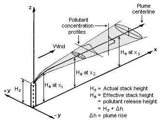
The Gaussian air pollutant dispersion equation (discussed above) requires the input of H which is the pollutant plume's centerline height above ground level. H is the sum of Hs (the actual physical height of the pollutant plume's emission source point) plus ΔH (the plume rise due the plume's buoyancy).
Visualization of a buoyant Gaussian air pollutant dispersion plume
To determine ΔH, many if not most of the air dispersion models developed between the late 1960s and the early 2000s used what are known as "the Briggs equations." G.A. Briggs first published his plume rise observations and comparisons in 1965.[7] In 1968, at a symposium sponsored by CONCAWE (a Dutch organization), he compared many of the plume rise models then available in the literature.[8] In that same year, Briggs also wrote the section of the publication edited by Slade[9] dealing with the comparative analyses of plume rise models. That was followed in 1969 by his classical critical review of the entire plume rise literature,[10] in which he proposed a set of plume rise equations which have become widely known as "the Briggs equations". Subsequently, Briggs modified his 1969 plume rise equations in 1971 and in 1972.[11][12]
Briggs divided air pollution plumes into these four general categories:
- Cold jet plumes in calm ambient air conditions
- Cold jet plumes in windy ambient air conditions
- Hot, buoyant plumes in calm ambient air conditions
- Hot, buoyant plumes in windy ambient air conditions
Briggs considered the trajectory of cold jet plumes to be dominated by their initial velocity momentum, and the trajectory of hot, buoyant plumes to be dominated by their buoyant momentum to the extent that their initial velocity momentum was relatively unimportant. Although Briggs proposed plume rise equations for each of the above plume categories, it is important to emphasize that "the Briggs equations" which become widely used are those that he proposed for bent-over, hot buoyant plumes.
In general, Briggs's equations for bent-over, hot buoyant plumes are based on observations and data involving plumes from typical combustion sources such as the flue gas stacks from steam-generating boilers burning fossil fuels in large power plants. Therefore the stack exit velocities were probably in the range of 20 to 100 ft/s (6 to 30 m/s) with exit temperatures ranging from 250 to 500 °F (120 to 260 °C).
A logic diagram for using the Briggs equations[5] to obtain the plume rise trajectory of bent-over buoyant plumes is presented below:
| where:
|
|
| Δh
|
= plume rise, in m
|
| F
|
= buoyancy factor, in m4s−3
|
| x
|
= downwind distance from plume source, in m
|
| xf
|
= downwind distance from plume source to point of maximum plume rise, in m
|
| u
|
= windspeed at actual stack height, in m/s
|
| s
|
= stability parameter, in s−2
|
The above parameters used in the Briggs' equations are discussed in Beychok's book.[5]
References
- ↑ J.C. Fensterstock et al, "Reduction of air pollution potential through environmental planning", JAPCA, Vol. 21, No. 7, 1971.
- ↑ C.H. Bosanquet and J.L. Pearson, "The spread of smoke and gases from chimneys", Trans. Faraday Soc., 32:1249, 1936.
- ↑ O.G. Sutton, "The problem of diffusion in the lower atmosphere", QJRMS, 73:257, 1947.
- ↑ O.G. Sutton, "The theoretical distribution of airborne pollution from factory chimneys", QJRMS, 73:426, 1947.
- ↑ 5.0 5.1 5.2 M.R. Beychok (2005). Fundamentals Of Stack Gas Dispersion, 4th Edition. author-published. ISBN 0-9644588-0-2. .
- ↑ D. B. Turner (1994). Workbook of atmospheric dispersion estimates: an introduction to dispersion modeling, 2nd Edition. CRC Press. ISBN 1-56670-023-X. .
- ↑ G.A. Briggs, "A plume rise model compared with observations", JAPCA, 15:433–438, 1965.
- ↑ G.A. Briggs, "CONCAWE meeting: discussion of the comparative consequences of different plume rise formulas", Atmos. Envir., 2:228–232, 1968.
- ↑ D.H. Slade (editor), "Meteorology and atomic energy 1968", Air Resources Laboratory, U.S. Dept. of Commerce, 1968.
- ↑ G.A. Briggs, "Plume Rise", USAEC Critical Review Series, 1969.
- ↑ G.A. Briggs, "Some recent analyses of plume rise observation", Proc. Second Internat'l. Clean Air Congress, Academic Press, New York, 1971.
- ↑ G.A. Briggs, "Discussion: chimney plumes in neutral and stable surroundings", Atmos. Envir., 6:507–510, 1972.
Further reading
- M.R. Beychok (2005). Fundamentals Of Stack Gas Dispersion, 4th Edition. author-published. ISBN 0-9644588-0-2.
- K.B. Schnelle and P.R. Dey (1999). Atmospheric Dispersion Modeling Compliance Guide, 1st Edition. McGraw-Hill Professional. ISBN 0-07-058059-6.
- D.B. Turner (1994). Workbook of Atmospheric Dispersion Estimates: An Introduction to Dispersion Modeling, 2nd Edition. CRC Press. ISBN 1-56670-023-X.
- S.P. Arya (1998). Air Pollution Meteorology and Dispersion, 1st Edition. Oxford University Press. ISBN 0-19-507398-3.
- R. Barrat (2001). Atmospheric Dispersion Modelling, 1st Edition. Earthscan Publications. ISBN 1-85383-642-7.
- S.R. Hanna and R.E. Britter (2002). Wind Flow and Vapor Cloud Dispersion at Industrial and Urban Sites, 1st Edition. Wiley-American Institute of Chemical Engineers. ISBN 0-8169-0863-X.
- P. Zannetti (1990). Air pollution modeling : theories, computational methods, and available software. Van Nostrand Reinhold. ISBN 0-442-30805-1.


