IS-LM model

The IS-LM model is used in the teaching of macroeconomics to depict the interaction of the factors determining the level of demand in an economy.

The Model

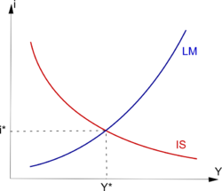
In its graphical form the model is shown as a pair of intersecting curves relating the level of national income (on the horizontal axis) to the rate of interest (on the vertical axis). The I-S (investment-savings) curve slopes downwards from left to right depicting the combinations of interest rate and savings that occur when the money market is in equilibrium. The L-M (liquidity - money supply) curve slopes the other way and depicts the combinations of interest rate and income level that make the demand for money equal to its supply.

The model includes two curves, IS and LM, in a graph in which the horizontal axis represents national income (Y) and the vertical axis represents the interest rate (i).

• IS illustrates the relationship between the level of income (Y) and the interest rate (i) in the real sector (goods and services). Lower is the interest rate higher is investment and thus the income.
• LM describes the relationship between the level of income and the interest rate in the monetary market. Higher is the level of income, higher is the need for money and thus the interest rate.

The intersection of the curves represents the general equilibrium for which both relationships are verified, that is to say the actual equilibrium of the economy.

The IS/LM model is the most common macroeconomic model. It enables to understand easily the relationships between the real sector and the monetary market as well as the short-run effects of monetary and fiscal policies. Yet its neglect of expectations makes it obsolete to determine the actual efficiency of macroeconomic policies.

History

Creation and rise

The IS-LM model creation is directly linked with the proposal by John Maynard Keynes of alternative assumptions to what classical economics assumed until then and seemed unable to explain the great depression. The main innovations in the General Theory were that prices were considered as rigid and money could be demanded for itself as an alternative to financial assets. Under those assumptions, the economy can be in equilibrium with a high level of unemployment whereas classical economics assumes that unemployment was regulated by variation in wages.

In 1937, John Hicks built the IS-LM model in order to translate those ideas in neoclassical terms. Some Keynesians saw his attempt as a simplification of Keynes vision but Keynes approved it.

The model summarized Keynes ideas in two curves. IS represented the equality between supply and demand in the goods and services market. The aggregate demand included consumption and investment. In the General Theory, consumption was a proportion of the income, called propensity to consume, while investment was related to interest rates. Variations of investment and consumption were amplified by the propensity to consume (spending multiplier). On the side of the monetary market, demand for money included speculative demand related to the interest rate and transactions demand related to the output while supply was controlled by the monetary authority.

The model demonstrated that under those assumptions, monetary and fiscal authorities could have a powerful influence on economic activity and thus reduce unemployment. It also provides a tool to understand and predict the effects of Keynesian policies. The IS-LM model knew the same future than Keynesian economics: rise and then decline.

An important extension of the IS-LM model was built by Robert Mundell (1963) and Marcus Fleming (1962) in the 1960's. The Mundell-Fleming model describes a small open economy with one more curve representing equilibriums of international exchanges.

Decline

During the 1950’s and 1960’s microeconomic investigations on consumption and investment gave a better understanding of the IS slope. Milton Friedman developed the idea that the consumption level of household’s was mainly determined by a long-term expectation a theory known as the permanent income hypothesis. Franco Modigliani life-cycle theory demonstrated that consumption was also related to age. Those two theories denied short-term policies to have an important effect on consumption, and thus the effects of the spending multiplier.

Such criticisms of keynesian ideas were not always criticisms of the IS/LM model. In fact, economists like Milton Friedman used the IS/LM framework to confute Keynesian economics. Yet Friedman rejected the paradigm of "general equilibrium" he viewed as characterized by "abstractness, generality, and mathematical elegance"

The most severe criticisms of the IS/LM model came from the fact that it negligees private agents expectations. Modern macroeconomic models which take expectations into accounts can provide results opposite to those of IS/LM. In fact, the model considers that short run is independent from long run. Yet expectations about the future have for example a direct impact on current wages which stimulates inflation and thus cancelled the positive effects of many macroeconomic policies described by the IS/LM model. In such cases, inflation remains the only effect and disturbs the coordination of private agents. The consequence of the rational expectations theory is that central banks of several industrial countries (the Federal Reserve and the European Central Bank for example) have been given independency and inflation control as their main objective.

Nowadays

Nowadays IS/LM model is an obsolete tool : its neglect of expectations makes it inefficient to implement an efficient economic policy. Yet, along with its Mundell-Fleming extension, it remains the most common macroeconomic model taught to undergraduate students because of its pedagogical qualities.

References

- ↑ Hicks, J. R. (1937), "Mr. Keynes and the Classics - A Suggested Interpretation", Econometrica
- ↑ Friedman, Milton (1957). A Theory of the Consumption Function. Princeton Univ Press.
- ↑ Bordo, Michael D. & Schwartz, Anna J. (2003), "IS-LM and Monetarism", National Bureau of Economic Research, p.18 [1]
- ↑ Milton Friedman (1949 (1953)), , "The Marshallian Demand Curve" in Essays in Positive Economics, Chicago: The University of Chicago Press, pp. 47-99.